Atmospheric absorption, spectra, units and code: companion page to the global warming explanation post
This is a companion page to my blog post on global warming (which is currently not yet ready).
I put up this post already as a teaser for my upcoming global warming post, which desperately needs expert review before I dare put it online. If you are an experienced climate/atmospheric scientist, would you please consider helping me out? Please email me on bert@hubertnet.nl if you can spare the time to skim my work for gross errors. The same goes for this page by the way!
On this page we’ll delve into the exciting subject of atmospheric absorption, spectra and the units used. We’ll also look at the code and databases behind the many graphs on the other page.
Absorption, spectra and units
To say the least, this is a confusing situation. It also doesn’t help that literature often papers over this by all too easily converting one kind of absorption unit into another one, without explaining how you can even do that.
The reason so many different units are used is that absorption is studied by different fields of science, and even within those fields, sub-areas of research are fondly attached to their own way of doing things.
In climate research, many of the separate practices of science come together, and it can be awfully confusing to see people juggle the favorite metrics from each field.
\[ \]Absorption by a specific gas (mixture)
We’ll start simple: we have a gas under certain conditions, and we’d like to describe how strongly it absorbs light of a certain frequency. This absorption causes attenuation of the beam, where attenuation could (by the way) also happen by other means. Attenuation is described as the (linear) attenuation coefficient, and is measured in units of \(cm^{-1}\), \(m^{-1}\), or even \(dB\cdot{}cm^{−1}\cdot{}MHz^{−1}\) for some reason. The neutron and nuclear crowd like to confuse us further by calling the attenuation coefficient the “macroscopic cross section”, which it is not.
So, if we have a \(cm^{-1}\) number for the attenuation coefficient, what does it mean? Again this depends on your field. Mostly, it means that if a beam traverses \(l\) centimeters of your material with attenuation coefficient \(\mu\), the absorbed fraction will be \(e^{-l\mu}\). Or in words, every \(\mu^{-1}\) centimeters, your beam attenuates by a factor of \(e\).

Graph showing the attenuation of light through a gas calculated using the attenuation coefficient
Some fields use decadal attenuation (\(10^{-l\mu_{10}}\)), and I hope let you know very clearly when they do.
Absorption by a material
We’d like to be able to calculate the absorption by a gas (mixture) from material properties. This turns out to be pretty hard even if you get the units right. But let’s start with the units.
The absorption properties of a material (at a certain frequency of light) are described as the Mass attenuation coefficient or the Molar absorption coefficient. The chosen units are \(m^2/kg\) or \(m^2/mol\). Square meters per kilo? How do we get from that to attenuation? The literature quickly assures us the latter easily converts to \(L\cdot{}mol^{-1}\cdot{}cm^{-1}\), but why? And what does that mean?
Square meter per kilo describes the cross section of the sum of all molecules in one kilo. That sounds like it sums the physical area of all the molecules, but it is not quite that. It is however the area of the shadow generated by molecules, or in other words, the area over which the molecules can catch light.
Under some circumstances, the mass attenuation coefficient of water is around \(1 m^2/kg\). This means that if we have a cubic meter of water vapor weighing 100 grams, and we shine light through it horizontally, 10% of that will be absorbed. The intercepting area of that 0.1 kilo of water is then equal to \(0.1 m^2\):

Slice from a 1 meter on a side cube, ~10% of light being intercepted. Blue circles represent some water molecules
If we compress this same amount of water vapor into a smaller volume, increasing the pressure, but decreasing the path length, nothing changes:

Slice from a compressed cube, ~10% of light being intercepted
The molar absorption coefficient works just the same, except per mol of a substance instead of per kilo. This also explains the alternate units for the molar absorption coefficient: \(L\cdot{}mol^{-1}\cdot{}cm^{-1}\). This can also be seen as \(cm^{-1}/(mol/L)\), and from there \(cm^2/(cm^3\cdot{}(mol/L))\). Since \(mol/L\) is the concentration, this is the molecular cross-section per 0.001 mol.
To convert the mass attenuation coefficient to the linear attenuation coefficient, we need to multiply it by the density of our material (\(kg/m^3, \rho_m\)). This turns the \(m^2/kg\) into \(m^{-1}\).
Intensities, line-based and continuum absorption
If we search for databases of absorption coefficients, or even mass attenuation coefficients, we won’t find these. What we do find are very long lists of intensities of ’lines’ in the spectrum of certain gases, plus a whole bunch of parameters that describe how these lines behave depending on pressure, temperature and the presence of other gases.
The most famous database of intensities is HITRAN. HITRAN is not just a database, it also comes with an Python based API to retrieve data from the web, and to turn these lines into actual spectra. The HITRAN project is 50 years old, and for continuity reasons uses a lot of (by now) odd units, like ergs and centimeter*kelvins. The hapi however will convert that for you to things like cm-1.
Converting the intensity of lines to an absorption spectrum is hard work, and it is good to know we can get the HITRAN hapi to do the heavy lifting for us. Because it turns out such lines broaden based on all kinds of parameters. Intuitively it makes sense that a fast moving molecule may experience light as a slightly different frequency based on the Doppler effect. And since the speed at which molecules move has a distribution, so does the absorption for a stationary line.
Doing calculations
In order to perform useful calculations on absorption, we need both the rotational-vibrational spectrum of gases, but for water also the continuum spectrum. You can get the first part from HITRAN (as mentioned above). The continuum spectrum can meanwhile be downloaded from the MT_CKD project.
Much of this data comes at a cadence that is not what you need. For example, the continuum spectrum is specified in 10 cm-1 intervals, whereas the line based spectrum really needs to be rendered in 0.01 cm-1 to capture the line shape. Also, the units are guaranteed to not to be compatible. A lot of this work is getting the wavenumbers and units right.
You can find the full Jupyter notebook on GitHub, but here are some key parts:
# let's fetch all the HITRAN we need
fetch('H2O',1,1,1,3500)
fetch('CO2',2,1,1,3500)
fetch('O3',3,1,1, 3500)
fetch('N2O',4,1,1,3500)
fetch('CH4',6,1,1,3500)
db_begin('data')
This uses the HITRAN API to retrieve the key gases. Note that ‘H2O’ etc is purely for convenience, in HITRAN you select molecules by their numbers (1, 2, 3 etc). We ask for data between wavenumbers 1 and 3500. HITRAN however does not have data for all gases down to wavenumber 1, some only start at 100. So there is work to do.
Here is a helpful function to get black body radiation in the right units for wavenumbers:
# v is wavenumber in cm^-1, T in Kelvin, output in W/m^2 for that frequency
def planckWNCM(v, T):
    v = v *100
    c = 3.0e8
    h = 6.62607015e-34
    kB = 1.380649e-23  # J/K
    return 100.0*math.pi*2.0*h*c*c*v*v*v/(math.exp(h*c*v/(kB*T))-1)
    # this is the power per square meter PER cm^-1 wavenumber, hence the 100 at the beginning
    # since planck law is in m^-1
This allows us to set up a Pandas DataFrame with a grid of wavenumbers, and representative outgoing longwave radiation (OLR):
layer = pandas.DataFrame({"nu": np.linspace(0.01, 3500, 350000)})
t=273.15 + 16
layer["inpower"]= layer.nu.apply(lambda x: planckWNCM(x, t))
This grid has a spacing of 0.01 cm-1. Next up is the key function that generated most graphs in the CO2 blog post:
def getGasAbsorptionPerMolecule(gas, ppmv, p=1., T=296.):
    nu,coef = absorptionCoefficient_HT(SourceTables=gas,
                                       Diluent={'air':1.0-ppmv/1000000.0, 'self': ppmv/1000000.0},
                                       Environment={'p':p,'T':T}, HITRAN_units=True)
    # cm^2/molecule
    df=pandas.DataFrame({"nu": nu, "coef": coef})
    df.set_index("nu", inplace=True)

    reindexed=df.reindex(df.index.union(layer.nu)).interpolate().
    fillna(0).reindex(layer.nu)

    if(gas=="H2O"):
        h2ocont=xr.open_dataset('MT_CKD_H2O/run_example/mt_ckd_h2o_output-radflag.nc')
        .to_dataframe()
        h2ocont=h2ocont.reindex(h2ocont.index.union(layer.nu)).interpolate().
        fillna(0).reindex(layer.nu)
        # cm^2/molecule
        reindexed.coef += (h2ocont.self_absorption).array

    return reindexed.reset_index()
This is the core function where it all comes together. We let the HITRAN API do the work to calculate the absorption coefficient in cm2 per molecule, using the Hartmann-Tran algorithm. We specify that we want to know what our gas does diluted in ‘air’, at a certain concentration.
Then on the ‘reindexed=’ line some Python Pandas magic happens to align the calculations from HITRAN to our wavenumber grid, and to fill out missing data. If HITRAN has no absorption data for a wavenumber (range) this means no absorption happens there, hence the fillna(0).
If we request the absorption for H2O, the continuum spectrum gets imported and also recast to our wavenumber grid.
Now, here is where it gets exciting. We read the H2O continuum spectrum from a netCDF file generated by a FORTRAN90 (yes) computer program from the MT_CKD project. And to make things a bit more exciting, you have to patch that project to create the right units:
--- a/run_example/mt_ckd.config
+++ b/run_example/mt_ckd.config
@@ -1,8 +1,8 @@
 &mt_ckd_input
        p_atm=1013.
-       t_atm=300.
-       h2o_frac= 0.00990098
-       wv1=497.
-       wv2=603.
-       dwv=1.
+       t_atm=296.
+       h2o_frac= 0.01
+       wv1=10.
+       wv2=3500.
+       dwv=0.1
 /
diff --git a/src/drive_mt_ckd_h2o.f90 b/src/drive_mt_ckd_h2o.f90
index 471a84c..58d6494 100644
--- a/src/drive_mt_ckd_h2o.f90
+++ b/src/drive_mt_ckd_h2o.f90
@@ -13,7 +13,7 @@
    double precision :: wv1,wv2
    real, dimension(:),allocatable :: sh2o,fh2o
    double precision,dimension(:),allocatable :: wvn
-   logical :: radflag=.FALSE.
+   logical :: radflag=.TRUE.

    integer :: nwv,i
    integer :: istat,ncid,id_wv,idvar(3)
This is needed to get the output in the right units, which happens by ‘including the radiation field term’. I’ve chased back papers to the 1970s to figure out what this means, but I still don’t get it. It does make the numbers come out correctly though. If anyone can explain this to me, I’d love to hear.
Next up, let’s have HITRAN calculate the absorption. This can take minutes since it has to take into account many other gases in the air:
#                                        ppmv
dfco2=getGasAbsorptionPerMolecule("CO2", 420, T=296, p=1)
dfh2o=getGasAbsorptionPerMolecule("H2O", 10000, T=296, p=1)
And finally we can make the big graph:
fig,ax =plt.subplots()
ax.set_yscale("log")

h2omolw = 0.018 # kg/mol
mw=h2omolw
df=dfh2o
#           m2/mol  / (kg/mol)  = (m2/mol) * (mol/kg) = m2/kg
conv=(1e-4*6e23*df.coef/mw) # *ppmv2kgpm3(420, 1000*co2molw)

ax2=ax.twinx()

r=conv.rolling(5000, center=True)
ax2.set_yscale("log")
ax2.set_yticks([100,10,1,0.1,0.01,0.001,0.0001,0.00001])
ax.set_xlim(0,3000)
ax.plot(df.nu, r.quantile(0.75), label='75% quantile')

ax.plot(df.nu, r.median(), color='black', label="Median")
ax.plot(df.nu, r.quantile(0.25), label='25% quantile')
ax.plot(df.nu, r.max(), ':', color='black')
ax.plot(df.nu, r.min(), ':', color='black')
ax.plot(df.nu, conv, alpha=0.2, lw=0.2)
ax.axhline(y=conv.mean(), ls=':')
ax.legend()
ax2.set_ylim(ax.get_ylim()[0]*ppmv2kgpm3(10000, 1000*h2omolw),
            ax.get_ylim()[1]*ppmv2kgpm3(10000, 1000*h2omolw))

ax.set_xlabel("wavenumber, $cm^{-1}$")
ax.set_ylabel("$m^2/kg$")
ax2.set_ylabel("$m^{-1}$")
plt.title("$H_2O$ long wave infrared absorbance, including the continuum spectrum, p=1 atm, T=296K, 40% RH")
And here is the graph:
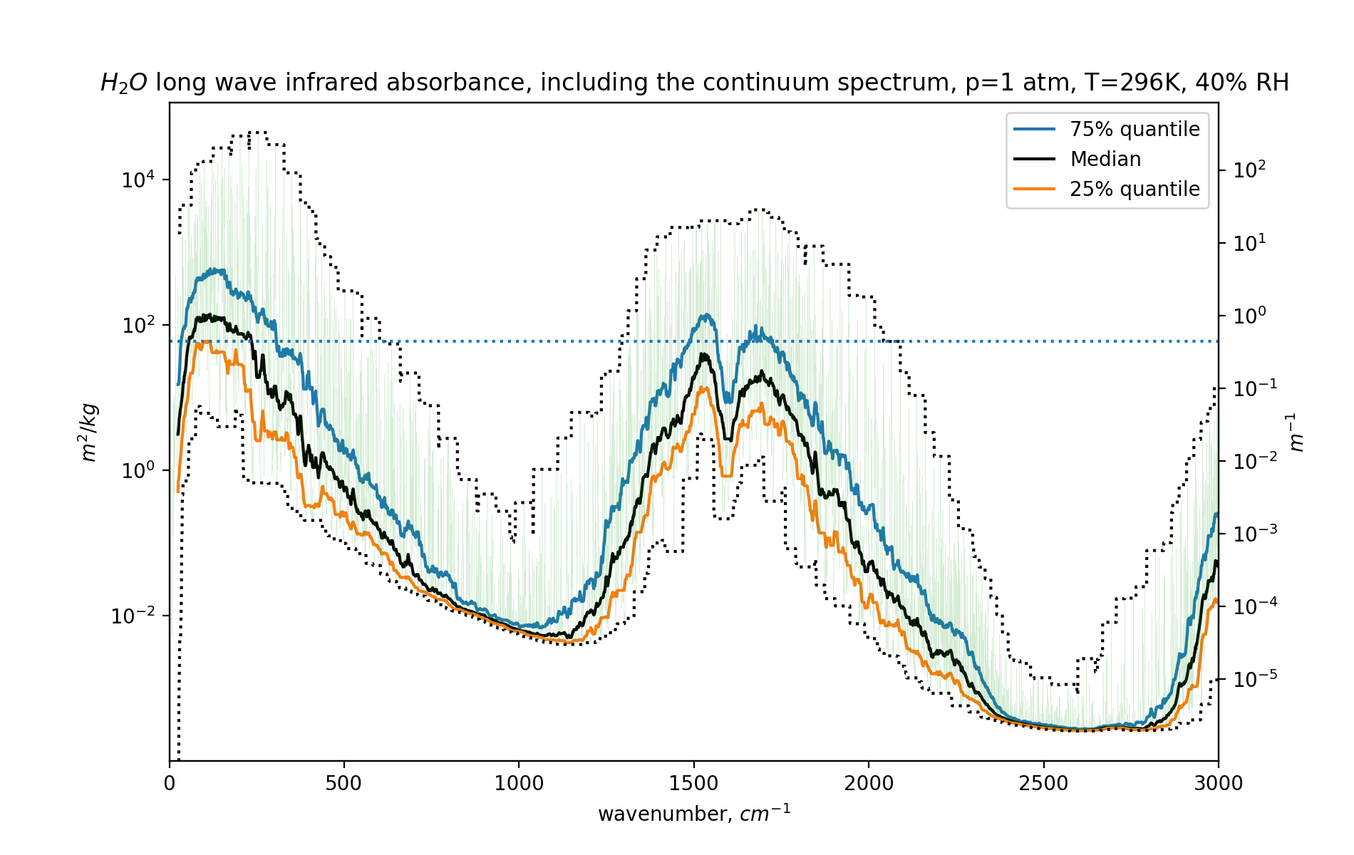
For far more details, do head to the GitHub repository.
Spotting serious research
Not all well-meaning climate research is great. And there is a large cast of characters that are writing articles meant to cast doubt on the human role in climate change. Sometimes the authors may seriously believe that, in other cases they may simply be grifting.
If someone sends you an article, here’s a checklist to see if it is serious science or not:
- Ignore the name or reputation of the magazine or website where the article was published. Really good science is frequently hard to publish in serious journals. And conversely, some truly abysmal stuff makes it to glam journals.
- If the article includes a homegrown radiative transfer model, it must come with source code. It is impossible to evaluate the outcome of an unknown model.
- Actually all papers with (novel) claims must come with open data and code
- Do they take the water continuum spectrum into account? If they don’t, no outcome can be reliable.
- If the outcome of a paper is that water vapor has a bigger effect than CO2, this is entirely correct. But do ask where that water vapor comes from.
- Time series analysis on recent data, always take a real good look at the years included. Do they just happen to miss out on an El-Nino? Or include Pinatubo? What would happen to the result with a few more years of data?
- There is no doubt about the validity of thermodynamics, so any paper that claims something in that regard is either Nobel prize winning material, or it is not serious (guess)